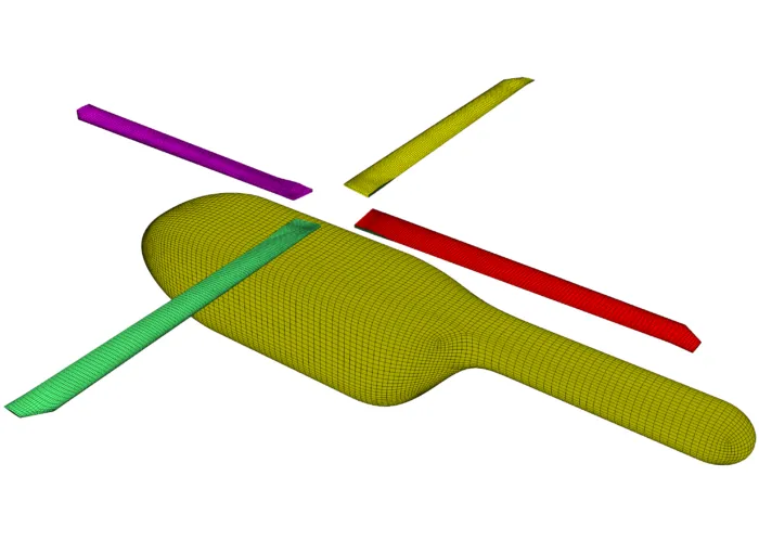
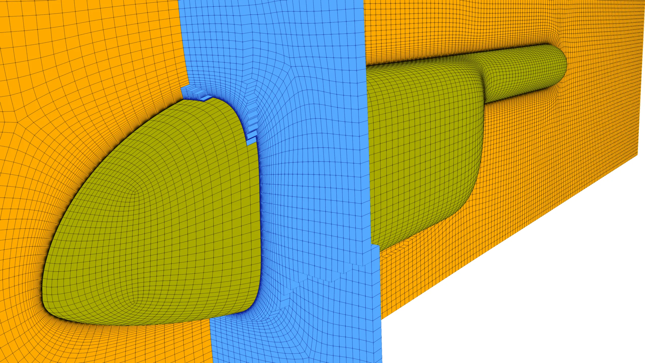
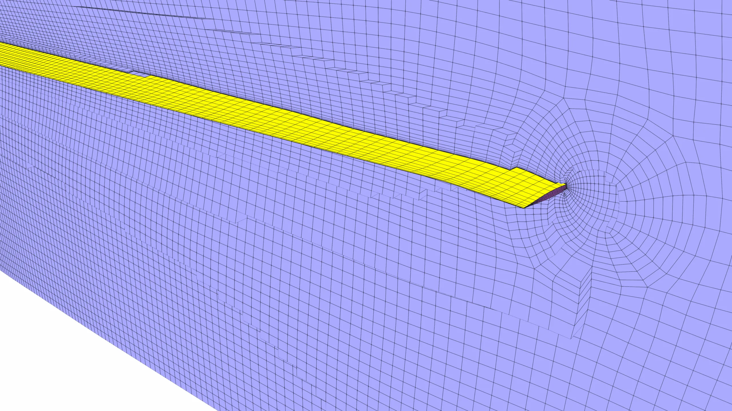
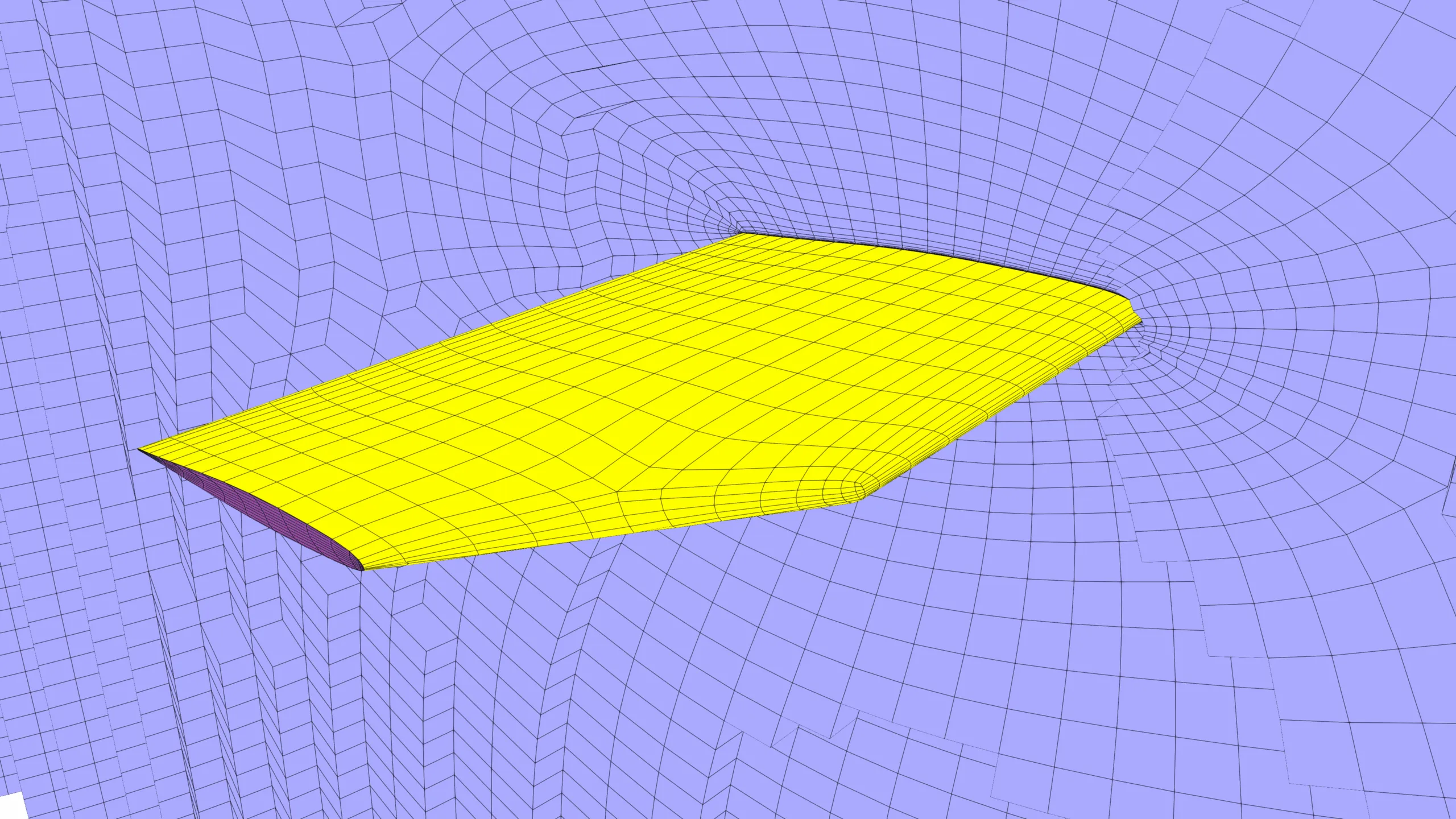
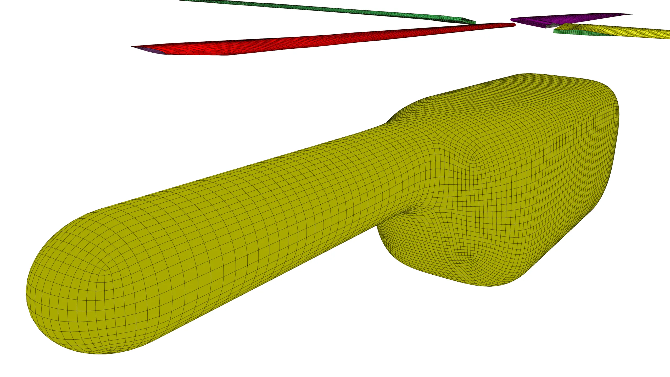
Figure 1: Structured hexahedral computational mesh generated for the Robin Helicopter rotor CFD simulation.
1570 words/ 8 mins read
Most helicopter rotor CFD simulations fail long before the solver converges. The real culprit isn’t turbulence modeling or residual plots, but a poorly designed mesh that destroys tip vortices before physics can emerge. Discover why topology, wake preservation, and near-body resolution determine whether your simulation predicts reality—or expensive aerodynamic fiction.
Imagine you are three weeks into a high-stakes rotorcraft project. The workstation is humming, the residuals on your Spalart-Allmaras turbulence model have dropped four orders of magnitude, and the lift curves look remarkably smooth. On paper, the simulation has “converged.” But when you calculate the Figure of Merit (FM), the number is 5% lower than the wind tunnel data. In the world of rotorcraft, a 0.5% error in FM is equivalent to the weight of an entire passenger. You have just realized your simulation didn’t just fail; it failed before the first iteration even began.
The “silent killer” in helicopter rotor CFD simulation isn’t the solver or the turbulence model—it is the spatial discretization, or more simply, the mesh. Most engineers spend 70% of their time tweaking solver settings and only 30% on mesh topology. For rotorcraft, this ratio must be reversed. In this deep dive, we explore why helicopter simulations are “vortex factories” and why your mesh is likely the reason your physics are vanishing into thin air.
The Physics: Life in a “Vortex Factory”
To understand the failure, we must understand the environment. Unlike fixed-wing aircraft, a helicopter rotor operates in a self-induced, three-dimensional flow field. Each blade sheds a powerful, highly concentrated tip vortex. These vortices don’t simply dissipate; they descend in a helical path, interacting with subsequent blades in a phenomenon known as Blade-Vortex Interaction (BVI).
The physical core of a tip vortex is incredibly small, typically only about 10% of the blade tip chord. If your mesh is not fine enough to resolve this tiny, high-gradient core, numerical diffusion will smear the vortex within less than half a revolution. When a diffused, “ghost” vortex strikes the following blade, the resulting pressure fluctuations are physically incorrect. This leads to the massive errors in performance metrics and aeroacoustic noise footprints that plague the industry.
The Structured Advantage: O-Grids, C-Grids, and the H-Grid Trap
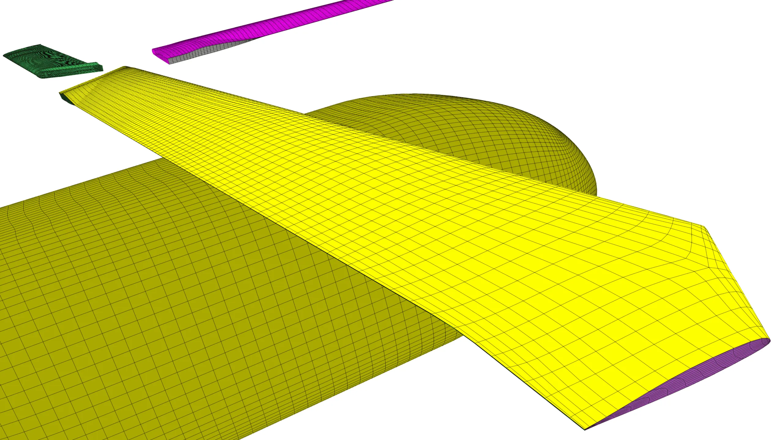
When it comes to rotor blades, not all cell arrangements are created equal. While automated unstructured meshing can reduce manual labor from weeks to hours, it often introduces significant numerical diffusion because it lacks the flow alignment necessary to preserve vortices. Topology-driven structured meshing remains the gold standard for high-fidelity results.
The O-Grid: Curvature’s Best Friend
Structured O-grids wrap coordinate lines continuously around the blade profile, providing excellent orthogonality at the solid boundaries. This is essential for resolving curved leading edges and capturing the secondary flows that develop in blade passages. However, O-grids have a fatal flaw for rotors: the grid lines loop back on themselves, causing rapid cell expansion downstream of the trailing edge. This coarsening “kills” the wake almost immediately, making O-grids poor for wake preservation unless they are combined with other topologies in a multi-block system.
The C-Grid: The Wake Preserver
A C-grid wraps around the leading edge but extends downstream from the trailing edge along a “split line” that naturally aligns with the wake. This topology is the hero of rotor CFD because it carries a high-density grid region exactly where the shear layers and vortices develop. It is particularly effective for resolving sharp trailing edges with minimal skewness.
The H-Grid: A Waste of Resources
While simple to construct, H-grids are highly inefficient for curved airfoils. Attempting to resolve a thin boundary layer with an H-grid propagates dense cell clustering far upstream into the freestream, wasting computational resources in regions where the flow is uniform.
The y+ Battle: Resolving the Viscous Sublayer
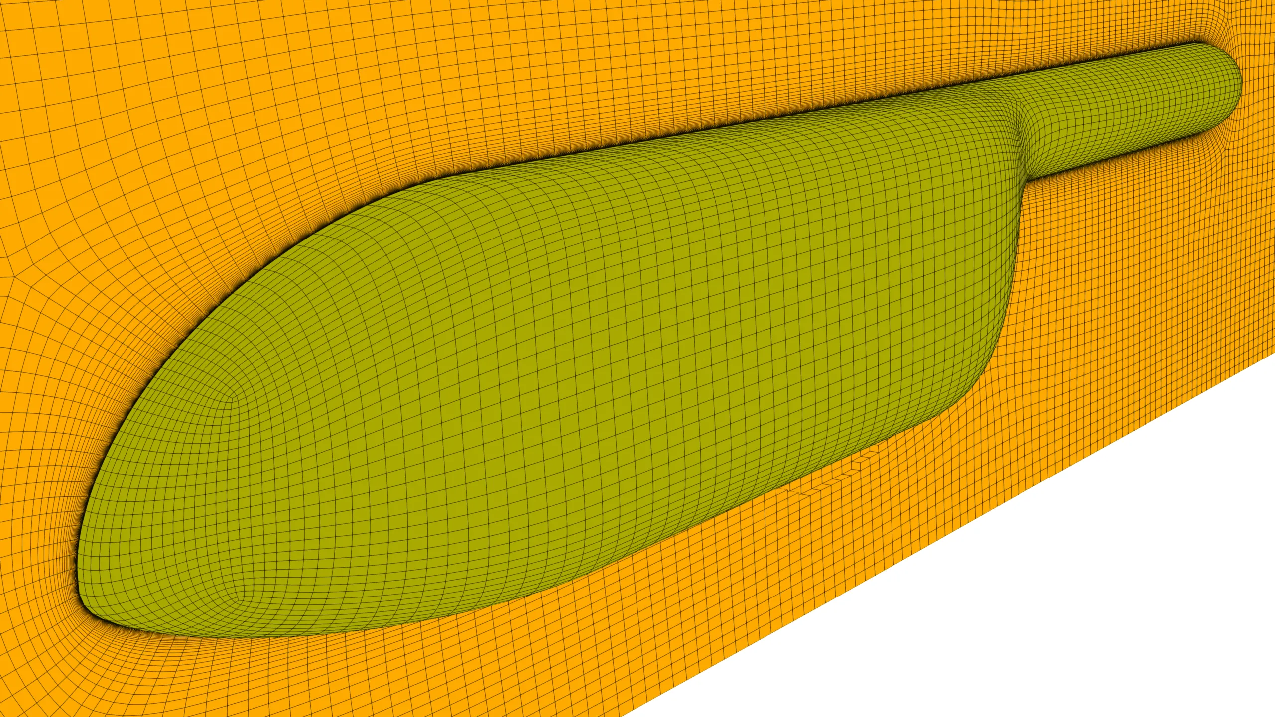
To accurately predict aerodynamic forces and phenomena like dynamic stall on the retreating blade, the grid must resolve the viscous sublayer. This requires a body-fitted, low y+ mesh where the non-dimensional wall distance of the first cell center satisfies y+ < 1.
For a typical helicopter rotor spinning at 2000 RPM, the high Reynolds numbers require an absolute first-cell height of 10-4 to 10-5 meters. If your mesh “skips” this sublayer, your skin-friction and torque predictions will be fundamentally flawed, and your Figure of Merit will never match experimental benchmarks. High-quality structured meshes achieve this orthogonality at the wall more efficiently than unstructured polyhedral or tetrahedral grids.
Modeling Motion: Sliding Mesh vs. Overset Assemblies
A helicopter rotor isn’t just a spinning fan; it is a complex kinematic system involving cyclic pitching, flapping, and coning to balance asymmetric loads. How you handle this motion in the mesh determines whether your simulation is robust or a numerical nightmare.
The Sliding Mesh (SM) Formulation
SM divides the domain into non-overlapping zones that rotate relative to one another along a shared interface. It is strictly conservative, meaning mass and momentum are perfectly preserved across the boundary. However, SM is limited to rigid, axis-aligned rotations. If your blade needs to flap or deform independently, the sliding interface—which must be a surface of revolution like a cylinder—becomes geometrically restrictive.
The Overset (Chimera) Mesh Approach
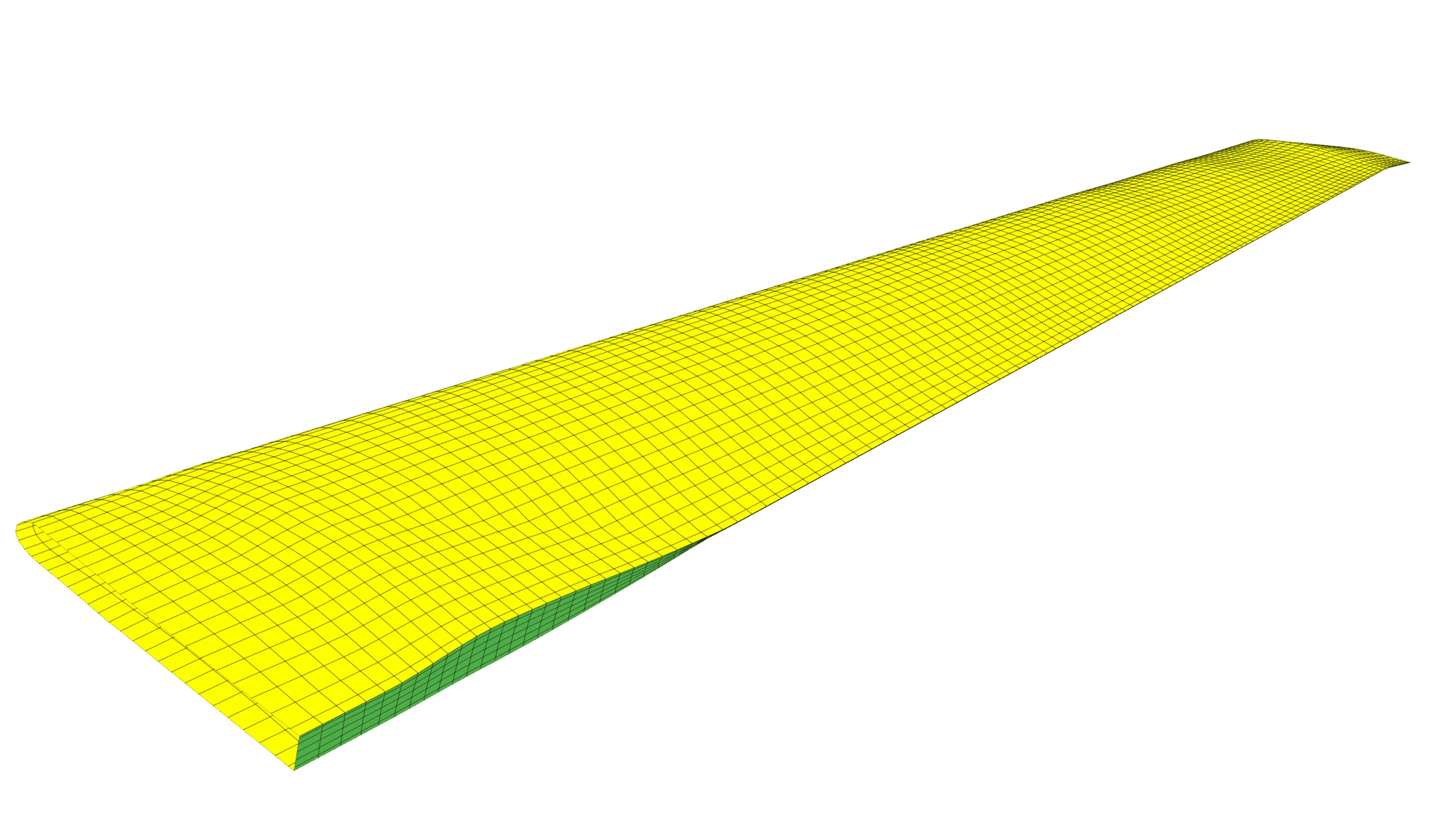
The industry standard for complex rotor kinematics is the Overset or Chimera method. This approach decomposes the domain into independent, overlapping sub-grids: a stationary background grid for the fuselage and individual near-body meshes for each blade.
These near-body meshes move freely across the background grid, allowing for arbitrary, multi-axis kinematics and structural deformations without requiring grid morphing. The catch? Overset grids are locally non-conservative. Variables are interpolated rather than flux-matched, which can generate spurious pressure oscillations if the cell sizes between the donor and receiver grids aren’t matched in the overlap region. To mitigate this, high-fidelity setups often use collar meshes—highly refined auxiliary grids that smooth the transition between overlapping components.
The Spatial Revolution: WENO Schemes and “Vortical Worms”
Even with a perfect mesh, standard second-order spatial schemes (like MUSCL) are often too dissipative for rotor wakes. To preserve the tip vortex over several revolutions, researchers have turned to 7th-order improved WENO-Z schemes. These schemes achieve high-order accuracy in smooth regions while preventing oscillations near shocks by dynamically shifting weights.
When you combine high-order WENO schemes with Adaptive Mesh Refinement (AMR) and Detached Eddy Simulation (DES), a unique physical phenomenon is revealed: vortical worms. These are small-scale, spinning secondary vortices that wrap helically around the primary tip vortices. For years, these were thought to be numerical artifacts, but they have recently been experimentally verified using Particle Image Velocimetry (PIV) by the German Aerospace Center (DLR). Capturing these worms is a hallmark of a high-fidelity simulation; they form through a process of entrainment and intense axial stretching of the blade’s trailing-edge shear layer.
The Figure of Merit Mystery: Near-Body vs. Off-Body Resolution
For over a decade, it was believed that poor wake resolution was the primary reason CFD under-predicted the Figure of Merit. However, landmark studies by Chaderjian and Buning at NASA proved that near-body grid resolution and spatial accuracy on the blade surface are actually more important for predicting FM than resolving the far-field wake.
In their tests, highly resolving the vortex wake reduced dissipation but did not significantly improve the FM. Instead, the accuracy was driven by getting the vortex strength right at the blade tip through fine body grids and high-order differencing. In fact, using 5th-order differences on a 35-million-point mesh yielded similar FM accuracy to a 3rd-order scheme on a massive 448-million-point mesh. This insight is a game-changer: it means you can achieve quantitative accuracy with fewer total points if you prioritize the mesh resolution directly on the blade.
Turbulence Modeling: Why Standard RANS Fails in the Wake
Standard Reynolds-Averaged Navier-Stokes (RANS) models, such as the one-equation Spalart-Allmaras, often fail in rotor simulations because they were designed for boundary layers, not free-stream vortices. In the rotor wake, the RANS length scale becomes the distance to the nearest wall, which can be several rotor radii away. This results in excessive Turbulent Eddy Viscosity (TEV), which artificially “melts” the tip vortices.
The solution is a hybrid RANS/LES approach like Detached Eddy Simulation (DES). DES uses RANS near the walls to resolve the viscous sublayer but switches to a more realistic LES length scale in the wake. This balances turbulent production and dissipation, preserving the helical tip vortices and allowing the physically realistic “vortical worms” to emerge.
Key Takeaways for Successful Helicopter Rotor CFD Simulation
If you want your helicopter rotor CFD simulations to succeed where most fail, remember these core principles:
- Topology is King: Do not just throw cells at the problem. Use structured C-grids for wake alignment and O-grids for leading-edge orthogonality.
- The Tip is the Key: The Figure of Merit is decided at the blade surface. Ensure your near-body mesh is high-order, tip-refined, and fully resolves the viscous sublayer (y+ < 1).
- Use Hybrid Turbulence Models: Switch from RANS to DES in the wake to prevent artificial vortex dissipation.
- Match your Interfaces: In overset setups, ensure your near-body and background grid cell sizes are identical in the overlap region to minimize non-conservative interpolation errors.
In helicopter rotor CFD simulations, the solver only computes what the mesh allows it to see. If you get the topology wrong, no amount of solver magic will bring the physics back. Start with a “Mesh-First” mindset, and the performance numbers will finally start to make sense.
Further Reading
- Meshing for Tip Gaps and Leakage Flows in Turbomachinery CFD
- How CFD Meshes Are Built for Modern Wind Turbine Blades: Why Structure Still Wins
- Fast and Accurate Hypersonic CFD Simulations: Impact of Automatic Shock-Aligned Meshes
References
- Chaderjian, N. M., and Buning, P. G., “High Resolution Navier-Stokes Simulation of Rotor Wakes,” (2011): This landmark study demonstrated that near-body grid resolution is more critical for predicting the Figure of Merit (FM) than off-body wake resolution, correcting a decade-long misconception in the industry.
- Chaderjian, N. M., “Advances in Rotor Performance and Turbulent Wake Simulation using DES and Adaptive Mesh Refinement,” (2012): This paper introduced the discovery of “vortical worms” (secondary vortices) and validated their existence through high-fidelity DES and AMR simulations.
- Mineck, R. E., and Gorton, S. A., “Steady and Periodic Pressure Measurements on a Generic Helicopter Fuselage Model in the Presence of a Rotor,” (2000): This is the definitive source for the NASA ROBIN (Rotor-Body Interaction) configuration, providing the experimental data used to validate virtually all modern rotorcraft CFD codes.
- Wolf, C. C., et al., “Experimental study of secondary vortex structures in a rotor wake,” (2019): This paper provided the first definitive experimental proof of the “vortical worms” predicted by CFD using tomographic Particle Image Velocimetry (tomo-PIV).
- Spalart, P. R., and Allmaras, S. R., “A One-Equation Turbulence Model for Aerodynamic Flows,” (1992): The foundational paper for the SA turbulence model, which is the most widely used closure in rotorcraft CFD simulations.
- Sun, Y., Shi, Y., and Xu, G., “Application of High-Order WENO Scheme… to Predict Helicopter Rotor Blade–Vortex Interaction Tonal Noise,” (2022): This work highlights the use of 7th-order WENO-Z schemes to minimize numerical dissipation and accurately capture BVI noise.
- François, et al., “Comparison of Chimera and Sliding Mesh Techniques for Unsteady Simulations of Counter Rotating Open-Rotors“: A critical comparative study that highlights the trade-offs between Overset (Chimera) flexibility and Sliding Mesh conservation.
- Steijl, R., Barakos, G., and Badcock, K., “CFD Analysis of Rotor-Fuselage Aerodynamics based on a Sliding Mesh Algorithm,” (2007/2009): This research developed and assessed algorithms for sliding interfaces in complex rotor-body configurations, focusing on efficiency and CPU overhead.
- Sankaran, V., et al., “Overview of the Helios Version 2.0 Computational Platform for Rotorcraft Simulations,” (2011): Provides a comprehensive look at the HELIOS dual-mesh paradigm, combining unstructured near-body grids with Cartesian off-body AMR.
- Lee, B. S., Jung, M. S., and Kwon, O. J., “Numerical Simulation of Rotor-Fuselage Aerodynamic Interaction Using an Unstructured Overset Mesh Technique,” (2010): A key paper for unstructured mesh validation using the ROBIN and UH-60 configurations.
- Chaderjian, N. M., “Quantitative Approach for the Accurate CFD Simulation of Hover in Turbulent Flow,” (2022/2023): This recent work synthesizes lessons learned over the last decade, providing a “quick-start” procedure and statistical measures for FM convergence in turbulent flow.