
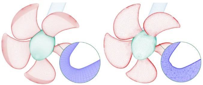
Figure 1: Structured multiblock grid for a marine propeller.
2600 words / 13 minutes read
Introduction
Like any other major engineering machine, ship propellers are always on the design table scrutinized for ways to improve their performance in terms of efficiency, noise characteristics, and erosion. New models are designed, performance analyzed, redesigned, and tested again. This cycle goes on, till a satisfactory design is obtained for a specific requirement.
The standard way to know the propeller performance is by model testing and CFD simulations. Called as open water performance analysis, a propeller is tested under wetted and cavitation flow conditions. Thrust, torque coefficient, and efficiency data are generated for various values of advanced ratio. Both experimental and CFD data are compared, verified, and validated to check the consistency in the data.
Compared to wetted flow, cavitation simulation is somewhat complicated due to strong interaction between numerical aspects such as grid density, timestep, cavitation, and turbulence model. In particular, modeling tip vortex cavitation is a challenging task, with the abilities of RANS codes tested to their limit while trying to capture the tip vortex flow accurately.
The article tries to address the gridding requirement for determining propeller open water and cavitation characteristics. Irrespective of the CFD solver in use, these gridding insights should aid in providing a better understanding of the relationship between grids, flow physics, and CFD solver.
Video 1: Sheet cavitation dynamics.
Domain and BC
Quite often, when not aware of the domain and gridding requirements for propeller simulation, individuals choose an arbitrary domain size and do multiple refinements to capture local flow dynamics. The refinement zone sizes are chosen based on intuition or prior experience or by trial and error. This arbitrary approach often leads to unnecessarily large domain and refined zone sizes leading to a large cell count. A mesh independent study with this set-up ends up being very expensive and time-consuming.
Typically, the domain shape chosen for open water propeller testing is cylindrical in nature. Taking the propeller diameter D as reference length, a cylinder of diameter 5D is constructed. The upstream inlet boundary face is placed at around 3D – 5D from the propeller while the downstream outlet boundary face is positioned at approximately 7D – 10D.
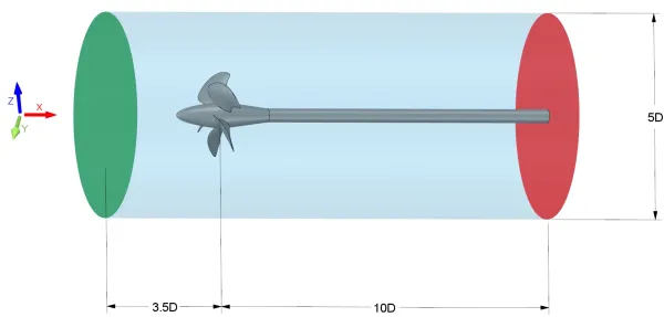
The domain dimensions are chosen to achieve a balance between theoretical requirements and evaluation time. The inlet boundary is moved upstream till a uniform flow ahead of the propeller is achieved, while the outlet boundary is pushed downstream to a location where reflections behind the propeller can be avoided and a fully developed flow is established at the outlet.

Computations for a single blade are also commonly performed. Propeller blades are periodic in nature and utilizing the periodic boundary condition, one can build a smaller domain, which significantly reduces the computational expenses.

Interface Modeling
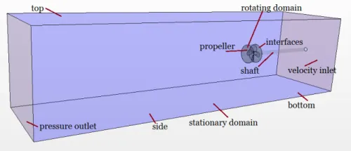
Usually, for propeller flow field computations the fluid domain is split into 2 zones. A zone closely around the propeller becomes the inner rotating zone and an outer zone called the stationary zone represents the rest of the domain. There are many ways to handle the fluid interaction through the interface between the two zones, out of which the most common ones are the moving reference frame (MRF) method, the mixing plane (MP) approach, and the sliding mesh (SM) technique.
Among these three, the sliding mesh technique being time accurate is considered to provide a completely strict solution but is unfortunately expensive in nature. Results generated using sliding mesh are in close agreement with the experimental data with respect to all integral characteristics. On the other hand, the quasi-steady moving reference approach and the steady mixing plane method can be considered as approximations of the exact time accurate solution. Each has its own advantages and disadvantages. Depending upon the simulation goal, time, and computational resources available, an appropriate method is chosen which to a larger or lesser extent meets the objective.
Simplified methods like MRF and MP have shown to accurately predict the integral forces on the propeller, but fall short in, accurate prediction of the amplitude of fluctuating forces. Further, it is observed that MRF and MP methods show sensitivity to the position of the downstream interface between the rotating and stationary mesh zones. In a nutshell, these simplified approaches provide higher accuracy when the interaction between the rotating and stationary domains are weak, but start to show their limitations in, flow conditions where there is heavy propeller loading and high propeller induced velocities in the slipstream.
In MRF and MP methods, the location of the downstream interface has an influence on the computational results, due to ‘numerical blockage’. If the interface is placed too close to rotating propeller blades, the interpolation of fluxes across the interface can generate disturbances in the flow, which show up in the velocity field of the propeller slipstream. Such disturbances are more noticeable when the mesh topologies on opposite sides of the interface are different. But when we position the interface sufficiently downstream of the blade, the disturbances disappear. This is because the vortex sheets leaving the blades now have sufficient space to develop before coming in contact with the interface. Now, a weak interaction is maintained between the domains separated by the interface and this arrangement improves the flow field predictive capability of the approach.
If one needs to strike a balance between accuracy and evaluation time, then, the moving reference frame method is the right one. With no physical movement of the computational grid, the computational time is reduced and the convergence also tends to be faster. The MRF model is a steady-state approximation in which individual domain zones move at different translational or rotational speeds. Rotation of rotating parts is included in the mathematical model by the addition of the centrifugal and Coriolis force. Unlike the transient simulations with a dynamic mesh, the MRF approach does not account for the relative motion of the moving zone with respect to adjacent zones (which may be moving or stationary). This means that the grid remains fixed during the entire computation. It is for this reason that MRF is often referred to as the ‘frozen rotor approach’.
Some researchers feel that although transient simulation is more accurate for propeller open water tests, they are of lesser importance since those results need to be averaged out in order to maintain the mean thrust and torque values required for open water curves. But for cavitation prediction, it is always better to go with transient simulation in order to achieve realistic results.
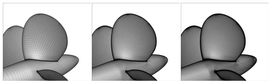
Figure 6: Sequential structured grids for a marine propeller. Image source ref [4].
Meshing Aspects for Marine Propeller
Once the domain dimensions and zone construction is complete, the focus can shift to discretizing the flow field.
Most propeller CFD analysis has a few things in common – a structure/unstructured/cartesian grid is generated, the grid is further refined sequentially or adaptively, and finally deployed for CFD computations. But the key element is, the solution accuracy largely depends on the adequate geometric representation and grid sensitivity in critical regions. Some researchers even go on to say that, if a mesh is defined appropriately, even the choice of the turbulence model has less of an impact on the final outcome.
A very common approach to propulsion prediction studies is to maintain a coarse mesh at the domain extremes and perform local refinement around the blades and in the axial direction in a cylindrical form with a diameter slightly larger than that of the propeller. Next, a grid-independent study is undertaken to ensure that the final solution is not dependent on the grid size. In this study, a gradual reduction in mesh size is made until the difference in thrust and torque coefficient values between two subsequent refined grids becomes small. Even the difference in the drag coefficient is also monitored until it is below 0.005 or less than 5 percent. However, sadly, even such a systematic gridding exercise may not certify that an optimum domain and refinement zones have been reached, but definitely improves the predictive quality of the whole CFD process.
When we look into the literature for the type of grids used for propeller analysis, we can observe that all gridding approaches from structured to unstructured to polyhedral and cartesian are regularly used for propeller domain discretization. The choice of the approach is usually based on the software usage skill, grid generator availability, time period allotted for meshing, and the level of accuracy expected. One or a combination of these factors influences the final decision-making process.
Nevertheless, irrespective of the approach, the fundamental gridding needs remain, the same – an adequate resolution to discretize the geometry features, proper resolution of the boundary layer, gradually coarsening of cells from the geometry towards the domain boundaries, and local refinement in regions of critical flow physics.

In marine propellers, the leading edge, the tip, trailing edge, and blade root are the critical regions, where important flow features develop and evolve. Sheet cavitation develops from leading-edge, tip vortex cavitation from blade tip, root cavitation from the root, etc, to name a few. Figure 7 shows all possible locations of cavitation for a typical propeller. So, the appropriate choice of mesh size, mesh type, and mesh structure, all become important in capturing these flow-rich regions.
Grid refinement can be done globally through generating sequential grids or it can be achieved locally through adaptive grid refinement. Local refinement allows for computationally efficient steady-state simulation.
In order to make optimized refinement, avoiding fine grids in unnecessary regions, local refinement is done. The leading edge, trailing edge and the tip of propeller blades have high curvature and are hence meshed with fine cells. This helps in capturing the geometry as well as the leading-edge suction peak. Further, the grids on the upper part of the blade as shown in figure 8 are refined as these areas tend to be of utmost importance when evaluating performance and analyzing cavitation. Also, in order to predict the tip vortex cavitation shape and extent more accurately, grid refinement is made in regions behind the blade, where cavitation rope is expected.
Marine propeller edges and tips are very thin with low radius and maintaining grid quality is a stiff challenge especially for structured grid-generators as it often results in the creation of highly skewed and twisted elements. So considerable attention needs to be given to mesh these tricky regions.

Adequate resolution of the boundary layer is also essential. For accurate flow prediction near the walls, boundary layer clustering with 30-40 layers is done with a fine first cell spacing with a y+ less than 1. Care should be taken to ensure that additional grid quality parameters like orthogonality and skewness are well within acceptable limits.

Wake refinement is done to capture the tip vortex. It is a recommended practice to do axial refinement along the propeller axis spanning the length of the domain with a diameter of 1.5D to 3D. Some researchers even go one step ahead and do an additional mesh refinement spanning the diameter of the external domain and extending axially for 0.5D to 2D, concentric to the propeller. Figure 10 shows wake grid refinement done for a marine propeller.
The mesh for the propeller performance prediction under cavitation conditions is more refined than that used for open water testing. For vortex cavitation cases with tip and hub vortex, further mesh refinement is necessary. One of the ways to do local refinement is by making use of a helical tube around the propeller’s tip as shown in Figure 11. Further, to capture the hub vortex accurately, another cylinder geometry can be used to create a volumetric control for capturing the extension of the hub cavitation as well. Figure 12 shows this refinement zone.

Performance of Structured and Unstructured Grids
Research shows that, in a certain range of advance ratios, structured and hybrid grids provide similar results, but at low and high ratios, structured grids tend to provide more accurate results.
Figure 13 – 14 shows the results of thrust and torque coefficients obtained on various meshes. For the advanced ratio in the range of 0.1 to 1.0, the numerical results are close to each other and compare well with experiments. The difference between results obtained using various meshes is less than 3 – 4 percent.
Figure 13: Relative errors in performance predictions for grids used in open water grid sensitivity study. Image source ref [2].
Overall results suggest that for a first cut quick numbers hybrid meshes are adequate to do performance prediction. But when a detailed investigation of the flow field is needed, hybrid meshes are not the right choice since they introduce excessive diffusion in the solution.

Both structured and unstructured grids can predict comparable levels of accuracy. So, depending on the requirements, one can opt for either of the two. If one is looking for speed and meshing simplicity then tet grids are the right choice. When using tets, it is essential to cross-verify whether the results are an outcome of cumulative numerical errors and incomplete geometric representation. An imposed grid size cap can lead to deficiencies, which might show up as numerical errors. However, the limitations of tet grids can be overcome by using hex-dominant or polyhedral unstructured grids.
If solution accuracy is the primary objective then structured grids are the preferred choice. With a structured approach, gridding challenges are easily eclipsed by multiple benefits – they are robust, an attribute clearly seen in cavitation tests, better geometric feature capturing capability with fewer cells, and are simpler to numerically solve leading to a significant reduction in overall computational time. Therefore, many recommend them as the right choice for marine propeller analysis.
Wrapping Up
With this, we come to the end of this article on gridding needs for open water propeller analysis. In the next article on marine propellers, we try to cover aspects of how the flow field prediction varies with grids, uncertainty analysis of wetted and cavitation flows, grid refinement study involving sequentially refined grids and adaptively refined grids, vapor volume uncertainty analysis, model vs full-scale performance analysis, etc.
Further Reading
- Multiblock meshing of Ship Propeller
- Influence of Mesh in Open Water Propeller CFD
- CFD Modelling of Submarine
- Cavitation in Turbines
References
1. “Comparison of Hexa-Structured and Hybrid-Unstructured Meshing Approaches for Numerical Prediction of the Flow Around Marine Propellers”, Mitja Morgut et al, First International Symposium on Marine Propulsors smp’09, Trondheim, Norway, June 2009.
2. “Grid Type and Turbulence Model Influence on Propeller Characteristics Prediction”, Ante Sikirica et al, Journal of Marine Science and Engineering, J. Mar. Sci. Eng. 2019, 7, 374.
3. “Numerical simulation of propeller open water characteristics using RANSE method”, Tran Ngoc Tu, Alexandria Engineering Journal, (2019) 58, 531–537.
4. “Computational fluid dynamics prediction of marine propeller cavitation including solution verification”, Thomas Lloyd et al, Fifth International Symposium on Marine Propulsors smp’17, Espoo, June 2017.
5. “Improving accuracy and efficiency of CFD predictions of propeller open water performance”, M. F. Islam et al, Journal of Naval Architecture and Marine Engineering, June, 2019.
6. “An Investigation into Computational Modelling of Cavitation in a Propeller’s Slipstream”, Naz Yilmaz et al, Fifth International Symposium on Marine Propulsion smp’17, Espoo, Finland, June 2017.
7. “A Numerical Study on the Characteristics of the System Propeller and Rudder at Low Speed Operation”, Vladimir Krasilnikov et al, Second International Symposium on Marine Propulsors smp’11, Hamburg, Germany, June 2011.
8. “Numerical characterization of a ship propeller”, Borna Seb et al, Faculty of Mechanical Engineering and Naval Architecture, University of Zagreb, Zagreb, 2017.
9. “Scale Effects on a Tip Rake Propeller Working in Open Water”, Adrian Lungu et al, Journal of Marine Science and Engineering, 2019, 7, 404.
10. “Cavitation on Model- and Full-Scale Marine Propellers: Steady and Transient Viscous Flow Simulations at Different Reynolds Numbers”, Ville Viitanen et al, Journal of Marine Science and Engineering, 2020, 8, 141.
11. “Energy balance analysis of a propeller in open water“, Jennie Andersson et al, Ocean Engineering, 158 (2018) 162–170.
12. “Developing Computational Methods for Detailed Assessment of Cavitation on Marine Propellers“, Abolfazl Asnaghi, Thesis for the degree of Licentiate of Engineering, Department of Shipping and Marine Technology, Chalmers University Of Technology, Goteborg, Sweden 2015.