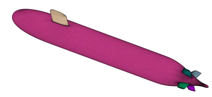
Figure 1: Structured multiblock grid for DARPA Suboff submarine CFD simulation

2159 words / 10 minutes read

Introduction

Submarines and Autonomous Underwater Vehicles (AUVs) have been in use for decades. While submarines predominantly are meant for military applications, AUV’s (visually looking like miniature submarines) have a wider range of applications. They are capable of performing a plethora of missions, including, under ice exploration, mapping and cable laying, pipeline and cable route survey and inspection, coastal survey and mapping, mine countermeasures, search and submarine hunting, hydrographic surveys, physical and chemical oceanographic survey, fish counting and environmental monitoring.

Though the areas of application of AUV’s have increased with time, their design and development cycle relying on traditional methods of model testing has been slow and expensive. However, with the advent of higher computing power and robust algorithms, CFD is rapidly emerging as a quick, reliable and economical design tool.

CFD in submarine design

In submarines and AUVs, any design thought is pivoted around two critical aspects of manoeuvring and speed-power performance. Whether its change in the contour of hull, sail, control surfaces or even the propulsion arrangement, the design decision-making process revolves around these two fundamental parameters. Other characteristics that the designer needs to pay attention to, like, the cavitation properties and the propeller noise radiation in deeply submerged, periscope and surface conditions.

In the early stages of design, investigations are made on the effect of change in size of control surfaces and sail, the effect of lengthening the hull by inserting new sections on the overall submarine manoeuvring characteristics, resistance and speed-power performance. Further, standard manoeuvres like zig-zag tests, turning circles and depth changes are also simulated to explore the effects of increase in control surface area, positional shift of sail in the longitudinal direction, inclination of the forward planes, etc. Later, in the advanced design phase, CFD runs are further made for transition location studies, analysis of propeller-hull interaction and scaling effects.

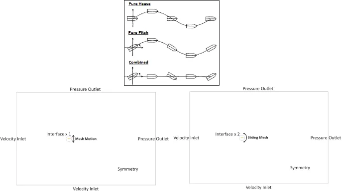
Animation 1: Different modes of ship motion. 

Need for hydrodynamic studies

Manoeuvrability plays a key role in the safe navigation and efficient service of a submarine. Unlike ships, submarines must be controlled in six degrees of freedom and require a complex set of control surfaces to meet the demands of its controllability. In order to evaluate the manoeuvrability of a submarine, the prediction of hydrodynamic forces and moments acting on the vehicle along with their derivatives in various modes of motion is essential.

To obtain these data, the submarine at design speeds is subjected to various modes of motion such as straight forward, drift, angle of attack, rudder deflection, circular and combined motion. Out of the many methods available to determine the hydrodynamics of a submarine, the captive model testing approach is considered as the most accurate method to determine all linear and nonlinear derivatives used for mathematical modelling of forces and moment. However, it has some demerits such as limitation of facilities, high cost of performance and scale effects.

In the last decade, CFD has emerged as one of the better options to predict hydrodynamics. Acting as a virtual captive model testing tool, CFD simulations help in computing the flow field utilising RANS or LES or DNS. Their accuracy, versatility and low cost make it an attractive tool.

Video 1: Submarine CFD: Captive model test at MARIN facility.

In this article, we try to cover the domain and meshing details of doing virtual captive modelling testing in CFD. It covers various aspects of domain shape and dimension, BCs, grid refinement and Y plus choices.

Hydrodynamic derivatives test cases

The standard captive model tests are conducted in water tanks to obtain hydrodynamic derivatives, which are also virtually replicated through CFD tools. Straight-line towing test, rotating arm test and planar motion mechanism test are the common ones.

Video 2: Straight-line towing test for a submarine hull.

Straight-line towing test

In a straight-line test, the model is towed in a straight line at a constant speed at various fixed incidences in a towing tank. The test is good to obtain static coefficients, but cannot determine angular or time-dependent velocities.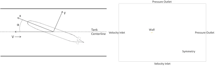 

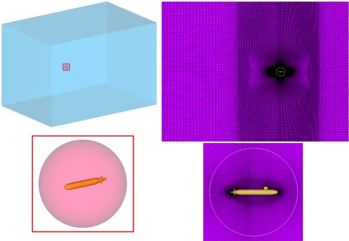
Figure 2: a. Straight-line towing test. b. BCs for towing test simulation. Image source [8].

Steady-state turbulent computations are done to replicate this test. A box domain as shown in Figure 2 is usually considered for simulating the test. The front, side and upper boundary faces are positioned at 15L [L = submarine length] from the model, while the outlet boundary face is placed at 25L from model. Dimensions are chosen with the intention of eliminating the effects of wall boundaries as well as flow reversals at the inlet/outlet boundaries.

Rotating arm test

This test is similar to straight-line towing test, except that the model is towed in a circular path in a larger towing tank with the longitudinal axis of the model either parallel or inclined at an angle to the circular path.

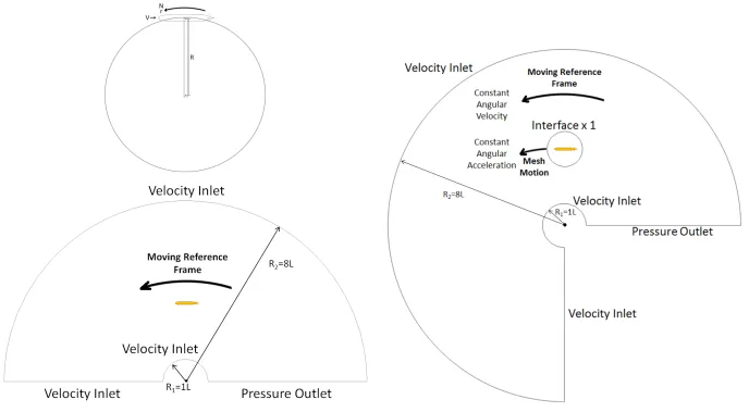
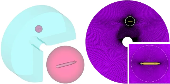
For the RA test simulation, the flow domain has a semi-cylinder shape with a hole at the center. The hole radius is L, the cylinder outer radius is 8L, while the cylinder height is 3L. Figure 4 shows the domain and boundary condition details. RA test is further bifurcated into two tests namely, constant angular velocity and constant angular acceleration.

Constant angular velocity

Study-flow simulations are performed by defining the entire domain as a moving reference frame cell zone. Figure 3b shows the domain and boundary conditions with no-slip BC applied for submarine wall, symmetry for side faces, inlet BC for front and bottom faces and pressure outlet BC for the back and top faces.

Constant angular acceleration

Figure 3c shows the domain and boundary conditions for RA constant angular acceleration test. The domain shape and the boundary conditions are similar to that in the constant angular velocity case, but, since the motion is time-dependent, transient unsteady simulation is needed. Also, the domain is split into two zones – inner and outer. The inner zone surrounding the submarine CFD model is allowed to move within the outer domain in a radial path. The boundary face common between the inner and the outer zone is defined with an interface BC.

Lastly, while moving reference frame cell zone condition is defined for the inner and outer domain, mesh motion condition is applied only for the inner domain. As the inner domain moves with time, the mesh for the outer domain is regenerated at each time step.

The same simulation can also be done using the spring analogy algorithm. The model is allowed to move in the domain, deforming the mesh. New node locations and the displacements on each node is calculated at each time step using the spring analogy while still maintaining the mesh topology.

Planar motion mechanism test

In this test, the model is towed at a constant speed in a towing tank, while been subjected to a sinusoidal motion at right angles to the axis of the towing tank. The longitudinal axis of the model may be parallel to either the axis of the towing tank or the direction of motion of the submarine.

The oscillatory motion can be pure yaw, pure sway, or a combination of the two motions on the horizontal plane. Similarly, on the vertical plane, the oscillatory motion can be pure heave, pure pitch, or a combination of the two.

PMM is considered as the most comprehensive test among hydrodynamic tests. Here all the derivatives namely velocity-dependent derivatives, rotary dependent derivatives and acceleration dependent derivatives can be obtained.

As far as the domain is concerned, for the pure heave case, a box domain shape having 2 zones with a common interface is used. For the combined motion simulation there is a slight modification. Two interfaces are used instead of one between the inner and the outer domain, with one belonging to the outer domain and the other belonging to the inner domain. Sliding mesh cell zone condition is imposed on the inner domain and mesh motion is also set for it. Unsteady analyses are conducted for all PMM simulations.

Gridding the submarine CFD flow field

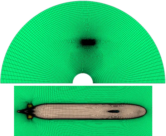
For discretising the flow domain, structured, unstructured gridding techniques including cartesian, overset approaches are routinely used. Volume grid refinement is generally done at regions of large flow variations such as the wake of the sail, wake of the propeller, and stern appendages. Mesh elements of finer size are placed in the wake area to capture details of the vortex structures.

While doing surface meshing care is taken to respect the geometric features and local flow physics. Usually, flow properties change considerably in regions where change in diameters occur and at locations of surface intersections. Therefore such locations are identified and finer surface mesh is used to capture them.

The viscous region in the near vicinity of the solid wall is captured by using a boundary layer padding. Depending on Y+ and turbulence model chosen, dense layers [~ 5-30] of cells are placed inside the boundary layer. Outside the padding, the cells are made to grow rapidly at a higher growth rate, as the far regions of the flow domain are less affected by flow changes around the model.

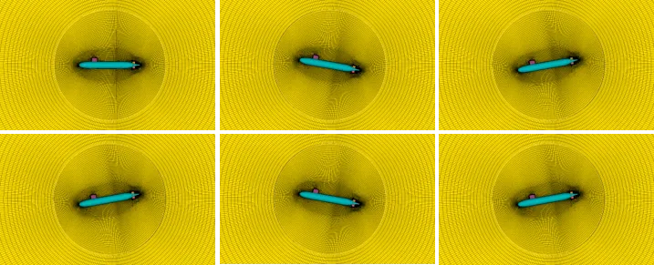
Video 3: Structured multi-block grids for DARPA Sub-off submarine CFD simulation.

If simulations are made considering the propeller along with the hull, the propeller surface is usually caged inside a cylindrical mesh zone. The cylindrical zone is free to rotate about the propeller axis. A sliding interface separates the cylindrical zone from the rest of the fluid domain.

For simulations with rudders, surface motions are accounted by using mesh distortion. As the rudder deflects to a new position with time step, the mesh in the structured block around the rudder gets locally deformed and smoothened out. With this, only a single grid will be necessary for the entire simulation instead of generating a new mesh for every instant of rudder position.

Typically around 45 percent of the cells are placed inside the boundary layer padding, another 40 percent of cells are distributed in the near vicinity of the submarine to capture the body wakefield and the rest 15 percent is used to discretize the farfield.

Determination of boundary layer mesh

The first spacing and number of layers in the viscous padding calculated based on Y+, depends on the turbulence model chosen and the computational expense one is ready to bear to conduct the simulation.

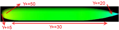
Figure 9 shows typical Y+ distribution for a submarine hull. On average Y+ is around 30. It reaches to a maximum of 50 near the bow, gets reduced to 10 within the separated region and drops further to around 5 at the leading stagnation region.

If low Reynolds number turbulence model like SA, k-omega, SST are chosen, then complete resolution of the boundary layer, including the viscous sublayer and buffer layer is necessary. The first cell spacing is calculated for a Y+ less than 1 and the boundary layer is finely packed with at least 25-30 layers. This large number of layers results in increased cell count and make the simulation computationally expensive.

On the other hand, turbulence models like standard k-epsilon are not low Reynolds number models. If they are chosen for performing the simulation, usage of wall function formulation is necessary. With wall functions, the flow field in the buffer region is ignored and an analytically computed nonzero fluid velocity is assumed. As a consequence, there is no more a need to completely discretise the viscous zone with fine first spacing and a large number of grid layers. This is a useful approach as it brings down the computational requirements significantly.

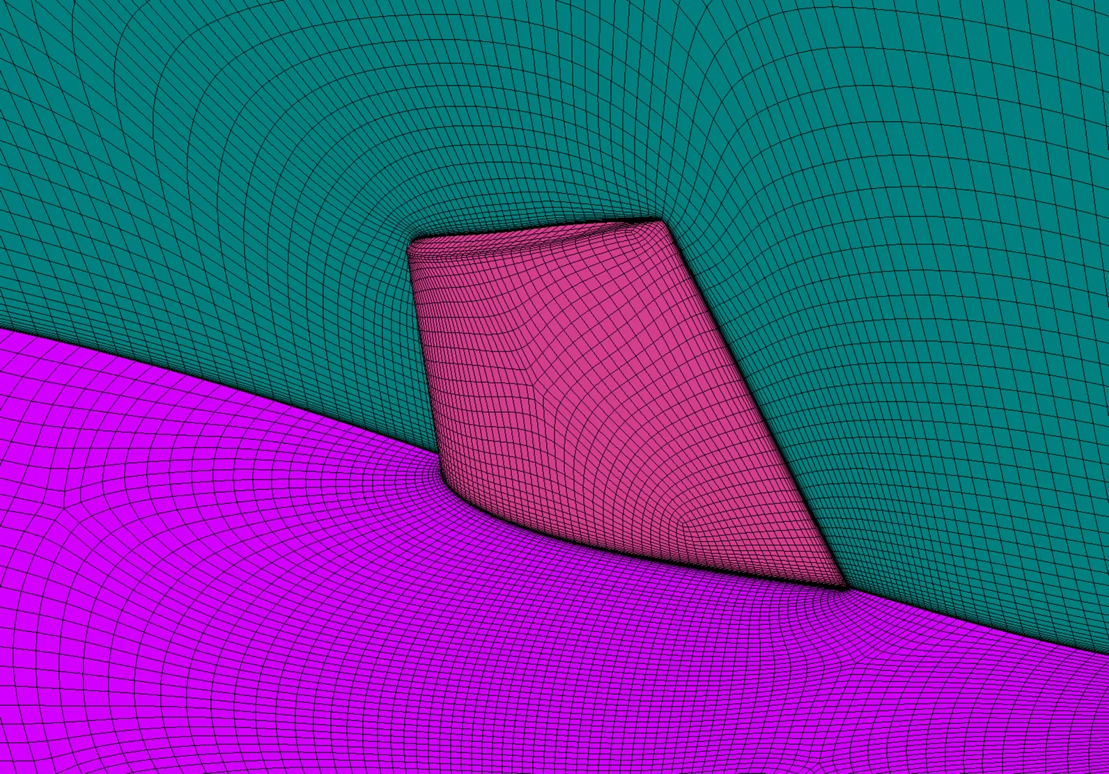
Figure 10 : Boundary layer clustering on the Hull and the Fin.

Certain flow solvers have automatic wall treatment functionality, which brings in the combined benefit of low Reynolds number models and wall function formulation. Depending upon the grid available, automatic wall treatment chooses which formulation to go with. For a dense boundary layer mesh, low Reynolds number formulation is used while for a coarse boundary layer mesh, wall function formulation is picked.

Interestingly, grid uncertainty analysis using various turbulence models has revealed that low Re wall modelling cases have a very good level of mesh convergence and very low resultant grid uncertainty levels compared to that will wall function modelling. Also, it is observed that automatic wall treatment formulation improves the mesh convergence and reduces the resultant grid uncertainty levels.

Parting thoughts

With this, we come to the end of this article. The grids used to discretise the domain may be anything from structured to unstructured, from cartesian to polyhedral. The domain and gridding requirements of submarines and AUVs are rather unique. The type of test determines the domain shape, number of zones, type of simulation – steady or unsteady. The key factor for the choice of the first cell spacing is based on the computational expense one is ready to bear to conduct the simulation.

Further Reading

1. Multiblock Meshing of Ship Propeller
2. RANS Based Automated Ship Hull Design Optimization

References

1. “Numerical Analysis of Wake Field over a Submarine with Full Appendages Based on STAR-CCM+”, Yichang Testing Techinque Research Institute, 2017 Joint International Conference on Materials Science and Engineering Application (ICMSEA 2017) and International Conference on Mechanics, Civil Engineering and Building Materials (MCEBM 2017) ISBN: 978-1-60595-448-6.

2. “Estimation of Hydrodynamic Derivatives of Full-Scale Submarine using RANS Solver”, Tien Thua Nguyen et al, Journal of Ocean Engineering and Technology 32(5), 386-392 October, 2018.

3. “Effects of Bulbous Bow on Cross-Flow Vortex Structures Around a Streamlined Submersible Body at Intermediate Pitch Maneuver: A Numerical Investigation”, Saeed Abedi et al, J. Marine Sci. Appl. (2016) 15: 8-15.

4. “Effective depth of regular wave on submerged submarines and AUVs”, Mohammad Moonesun et al, Volume 2 Issue 6 – 2017, International Robotics & Automation Journal.

5. “CFD RANS Simulations on a Generic Conventional Scale Model Submarine: Comparison between Fluent and OpenFOAM”, D.A. Jones, Maritime Division, Defence Science and Technology Group, DSTO-TN-1449.

6. “Numerical Simulation Study on the Effects of Course Keeping on the Roll Stability of Submarine Emergency Rising”, Shudi Zhang et al, Appl. Sci. 2019, 9, 3285.

7. “Simulations of the DARPA Suboff submarine including self-propulsion with the E1619 propeller”, Nathan Chase, MS (Master of Science) thesis, University of Iowa, 2012.

8. “Numerical Simulation Of Hydrodynamic Planar Motion Mechanism Test For Underwater Vehicles”, Mustafa Can, The Graduate School Of Natural And Applied Sciences Of Middle East Technical University, September 2014.

9. “Simulations of a Self Propelled Autonomous Underwater Vehicle”, Alexander Brian Phillips, Thesis for the degree of Doctor of Philosophy, University Of Southampton Faculty Of Engineering, Science & Mathematics, April 2010.

10. “Use of computational fluid dynamics as a tool assess the hydrodynamic performance of a submarine”, P.G. Marshallsay et al, 18th Australasian Fluid Mechanics Conference”, 3-7 December 2012.

Subscribe To GridPro Blog