Influence of Meshes on Hydraulic Turbines CFD GridPro Blog

Figure 1: Structured multi-block grid for Hydraulic Francis turbines

1850 words / 9 minutes read

This is the 3rd article in the series on Hydraulic Turbines:

Part 1 – Understanding the flow through Francis turbine.
Part 2 – Know the Flow – Cavitation in hydraulic turbines.
Part 3 – Influence of Meshes on Hydraulic Turbine CFD.
Part 4 – Grid Convergence Study for Francis Turbine- From a Meshing Software Perspective.

Introduction

In continuance to our previous articles on the flow physics in Francis turbines and cavitation effects. In this article, we discuss on the numerical prediction of the flow features and performance of a hydraulic turbines. The numerical prediction depends on a number of factors including domain model, mesh, turbulence model, boundary conditions, etc. While influential factors like domain modeling, mesh creation are taken care of in the preprocessing stages, aspects like turbulence model and boundary conditions are addressed during the solver run stage. But domain modeling and grid generation are something that influences even the turbulence model chosen and the boundary conditions applied to do the simulation.

There are various grid types that are used to discretize the hydraulic turbine flow field. Structured hex grids, unstructured grids with prisms and tets are the most common ones. Hybrid grids comprising of tets, prisms in complex regions and structured hex cells in geometrically simpler reasons are also quite popular. Adaptation of the base grids is also done to get refined grids for accurate capturing of the geometry and flow features.

Grid and the flow domain model selected influences the predicted flow solution in varied ways. In the following sections, we try to cover these aspects in detail starting with domain modeling and followed later with grid convergence and the effects of grid density on the flow field.

Modeling Approach

Fluid domain modeling for numerical simulations of turbine flows can be done in three ways, namely, complete turbine modeling, components based modeling and passage modeling.

In the complete turbine modeling approach, the outer volute, the stay vanes, guide vanes, runner with blades and splitters and draft tube are modeled. In component modeling, the runner and draft tube alone is modeled. And in passage modeling, the flow passage of the distributor and the runner blade with splitters are modeled.

Each approach has it’s own advantages and disadvantages. The complete turbine approach is expensive compared to the other two approaches. Results from the complete turbine and component modeling approaches are quite similar without many significant differences. Also, it is considered that, if accurate boundary conditions are prescribed than the component modeling approach can provide an optimum solution.

On the other hand, the passage modeling approach helps in reducing the computational power and time. It generates good results but does not take into consideration the influence of the flow variations in the neighboring passages. However, there has been some recent developments in passage modeling which is considered to provide reliable results in hydraulic turbines, including dynamic pressure pulsations generated by rotor-stator interaction.

Even before we go into the newer passage modeling approach, let’s try to understand the conventional passage modeling approach a bit better. In a conventional approach, a blade and a guide vane passage is modeled. This approach has some demerits as it introduces errors at the interface when the flow variables are averaged out. As a consequence, the flow unsteadiness are not resolved. This approach generates accurate results when the pitch ratio between the modeled stator and rotor passage is equal to 1.

Now pitch ratio in simple terms means, the ratio of the circumferential angle or length of the modeled guide vane to that of the blade passage. Since in water turbine designs the number of guide vanes and blades are consciously chosen to avoid a common denominator to avoid instabilities, it is very difficult to get a case with a pitch ratio of 1 for numerical investigation.

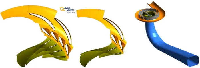
Blade torque in a Francis turbine. — **Figure 3:** Variation in the blade and splitter torque in a Francis turbine under BEP operating
*conditions; PT-profile transform, FT-Fourier transform, 360-complete turbine modeling. Image source Ref [1].*

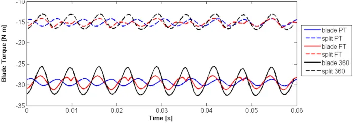
Interestingly, a novel technique making use of Fourier transformations has been developed to model the flow passages without limiting the pitch ratio. In this approach, two flow passages around a blade with splitter are considered with a pitch ratio of 0.933 as shown in Figure 2a. To check the relative performance, computations were done with the two passage modeling along with one passage modeling and the complete turbine modeling. Figure 3 shows the maximum blade torque amplitude under best efficiency point conditions for the three approaches.

The complete turbine approach predicted maximum amplitude while the single passage profile transformation approach predicted the lowest. The two passage Fourier transform approach showed an amplitude intermediate to that predicted by the complete turbine and single passage approach. This means that the Fourier transformation technique does a better prediction than the profile transformation approach when the pitch ratio is not unity. In a way, this approach is a compromise between the numerical accuracy and computational power required to simulate the complete turbine.

**Figure 4:** Pressure distribution on the blade for three grid densities and extrapolated pressure. Image source Ref [1].

Ways to Determine Independency of the Solution on the Mesh

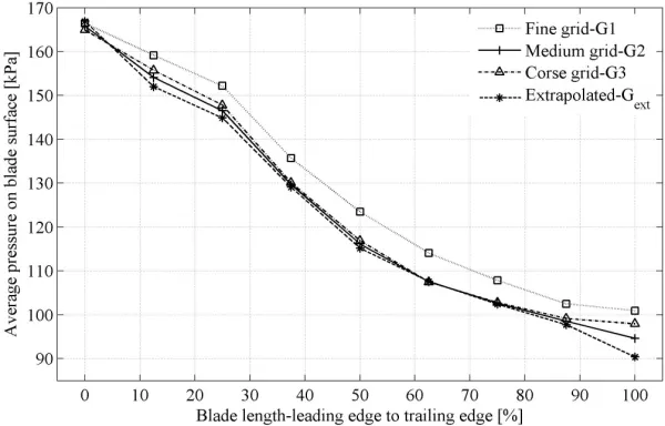
Whenever an exercise to do computation for hydraulic turbines is undertaken it is a good practice to do a grid convergence study to pick one optimal grid to do production runs. Figure 4 shows one such mesh scaling test conducted by the organizers of the Francis-99 workshop with three structured grids of sizes 20, 10 and 5 million nodes. The fine grid shows a maximum discretization uncertainty of 5.81 percent at the blade trailing edge while the medium grid showed a maximum uncertainty of 4.1 percent. The predicted hydraulic efficiency from the medium grid was closer to the experimental value and was hence distributed among the participants as a standard grid for production runs. Sometimes other parameters such as output power are also used as a variable to decide the grid resolution.

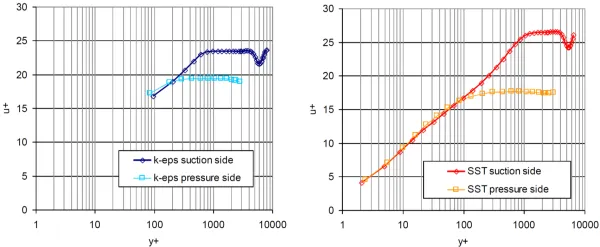
**Figure 5:** Boundary layer estimation on the pressure and suction sides of the guide vane with different y + values and turbulence models. Image source – Ref [1].

Apart from the overall grid size, it is observed that y+ value and grid resolution in the boundary layer affects the flow field. For example, it is noticed that, for a simulation with SST turbulence model, the computed power is dependent on the y+ value of the first cell thickness. Figure 5 shows the near-boundary velocity variation on the pressure and suction sides of a guide vane for the different values of y+ and turbulence models. So choosing the right first spacing is also another factor to take into account while trying to make the solution grid-independent.

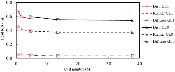
**Figure 6:** Head losses in the turbine for the three mesh densities at two different grid levels. Image source – Ref [1].

Another effective way to determine the independency of the solution on the mesh is by analyzing the head loss variation at the distributor stage, runner stage and draft tube stage with cell count. Generally, the head loss prediction improves with grid density. For a coarse grid of about one million nodes, the head losses at the three stages of a turbine like the distributor, runner and diffuser are typically predicted high as can be seen in Figure 6. Loss in head reduces with an increase in grid density. However, there is no significant difference in head losses with grid refinement in excess of 13.48 million nodes. Hence a grid size of 13.48 million was chosen as the optimal grid with 5.1, 6.3 and 2.08 million nodes in the distributor, runner and draft tube respectively. This chosen mesh exhibited numerical errors of 1.7 percent, 0.6 percent and 0.4 percent for the distributor, runner and draft tube respectively.

**Figure 7:** Hydraulic turbines: Vortex rope as captured by a coarse mesh. Image source Ref [4].

Pressure Pulsation Amplitude Prediction

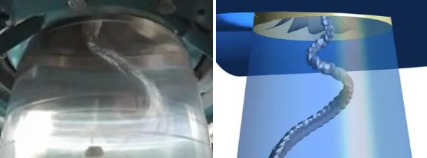
Acurate capturing of critical flow parameters like the amplitude of pressure pulsation due to the rope vortex in the draft tube also varies with the grid resolution. If the grid is coarse, the vortex rope cannot be captured accurately. Figure 7 shows an attempt by a coarse grid to capture a vortex rope. The staircase-like structure is due to insufficiently refined mesh in the vertical direction.

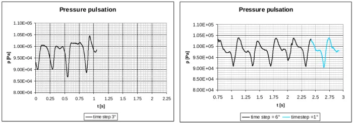
Hydraulic turbines CFD: Pressure pulsations for part load operating points with two computational grids: a - 3.3 M elements, b - 17 M elements. — **Figure 8:** Hydraulic turbines CFD: Pressure pulsations for part load operating points with two computational grids: **a –** 3.3 M elements, **b –** 17 M elements. Image source – Ref [5].

Figure 8 presents the pressure pulsation amplitude for a coarse 3.3 million grid and a finer 17 million grid. For the coarse grid, the time step is 3 degrees of runner revolution and for the fine grid, the first part of the graph shows time step of 6 degrees while at the end it is 1 degree. The difference in the frequency and amplitude due to time step are negligible but that due to grid resolution can be clearly seen. The amplitudes of pressure pulsation on the fine grid are significantly higher than those on the coarse grid.

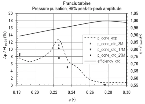
**Figure 9:** Pressure pulsation amplitudes for different operating regimes; comparison between experimental and numerical values. Image source – Ref [5].

When we compare the CFD predicted pressure pulsations amplitude with experimental results, the differences can be more than 50 percent with a coarse 3.3 million grid in the operating regime. With a finer 17 million grid, the differences are less than 10 percent. Figure 9 shows the plots comparing the numerical results with experiments.

Hydraulic turbines: Velocity distribution on mid-cross-section at BEP — **Figure 10:** Hydraulic turbine: Velocity distribution on mid-cross-section at BEP. Image source [6].

Flow Energy Loss in the Distributor, Runner, and Draft Tube due to Grid

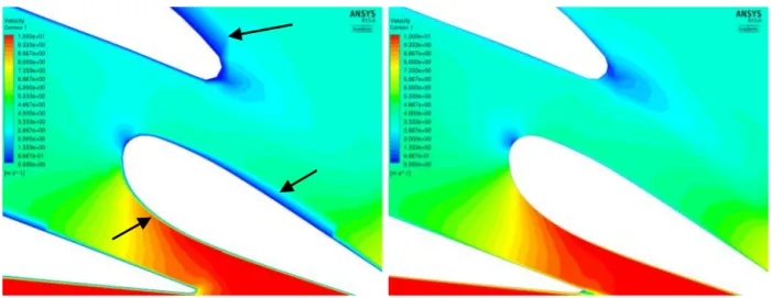
Flow energy losses in the volute, stay and guide vane are greatly influenced by the grid resolution. Sufficient grid density around the vanes is crucial for accurate prediction of frictional losses. Figure 10 illustrates the velocity fill plot for a coarse grid and a fine grid in the distributor. As can be observed, the grid in the vicinity of the stay and guide vanes including the boundary layer is not properly refined. The abrupt changes in the velocity field in the boundary layer (kinks) are the clues to the gridding mistakes. As a consequence, the flow energy losses calculated on the coarser grid is larger than that on a finer grid. The influence of grid refinement on losses is more significant at part load conditions where guide vane openings are small and velocity large. It is reported that the energy losses in the distributor at part load can be as high as 4.6-4.9 percent of the head, while that at BEP and high loads are around 4 percent and 3 percent respectively.

The pressure field around the runner blades is greatly influenced by the grid resolution around it. Too large a y+ results in a much larger runner head and shaft torque prediction. Due to both these effects, smaller flow energy losses in the runner were obtained for the coarser grid than on the finer grid. Interestingly, this difference is quite large at part load, while it is insignificant at BEP and high load conditions.

Trailing Thoughts

The quality and accuracy of prediction on a given grid depend on the flow solver used as well. A mesh will not provide the same results for different codes. The final solutions are a function of the code used as well and each code operates differently. It is for this reason that in international workshops like Francis-99, that even though the organizers provide carefully crafted structured grids to the participants, the participants either generate their own grid with an improved quality or tweak the organizer’s grid to suit their solver needs. Systematic quantification of the mesh parameters, minimum angle, volume change, aspect ratio, etc could help in the standardization of the grids. This could tremendously aid in making the grids inter-code compatible and hopefully also make codes generate near-same results on a common grid.

This brings us to the end of Part 3 in the Series on Hydraulic Turbines. In the fourth and final article in the series, titled, Part 4 – Grid Convergence Study for Francis Turbine- From a Meshing Software Perspective we try to cover aspects of generating a sequential grid family for doing grid convergence studies.

Hydraulic Turbine Series:

Reference
1. “Experimental and Numerical Studies of a High-Head Francis Turbine: A Review of the Francis-99 Test Case”, Chirag Trivedi et al, Energies 2016, 9, 74; doi:10.3390/en9020074.

2. “Numerical prediction of pressure pulsation amplitude for different operating regimes of Francis turbine draft tubes”, Andrej Lipej et al, International Journal of Fluid Machinery and Systems Vol. 2, No. 4, October-December 2009.

3. “Numerical prediction of the vortex rope in the draft tube”, DRAGICA JOŠT, 3 rd IAHR International Meeting of the Workgroup on Cavitation and Dynamic Problems in Hydraulic Machinery and Systems, October 14-16, 2009, Brno, Czech Republic.

4. “Numerical Prediction of Cavitating Vortex Rope in a Draft Tube of a Francis Turbine with Standard and Calibrated Cavitation Model”, D Jost, IOP Conf. Series: Journal of Physics: Conf. Series 813 (2017) 012045.

5. “Numerical Prediction of Non-Cavitating and Cavitating Vortex Rope in a Francis Turbine Draft Tube”, Dragica Jost et al, Journal of Mechanical Engineering 57(2011)6, 445-456.

6. “Numerical simulation of flow in a high head Francis turbine with prediction of efficiency, rotor stator interaction and vortex structures in the draft tube”, D Jost, Journal of Physics: Conference Series 579 (2015) 012006.

7. “Numerical Simulation of Three-Dimensional Cavitating Turbulent Flow in Francis Turbines with ANSYS”, Raza Abdulla Saeed, International Journal of Aerospace and Mechanical Engineering Vol:9, No:8, 2015.